A recent study by Feiveson et al. ![]()
![]() establishes the Federal Open Market Committee's interest in the distributional effects of monetary policy. The size and the composition of household income exhibit large variation over the life cycle, so it is likely that household exposures to monetary policy also depend on age. This post summarizes new research by Daisuke Ikeda and me that uses a life cycle model to measure the age profile of household exposures to monetary policy. In the model, a higher nominal interest rate increases the wealth and consumption of households between the ages of 60 and 80, but it reduces the wealth and consumption of younger working-age households and the oldest retirees. The former group also has the highest net worth, and it follows that net worth and consumption inequality increase in the model.
establishes the Federal Open Market Committee's interest in the distributional effects of monetary policy. The size and the composition of household income exhibit large variation over the life cycle, so it is likely that household exposures to monetary policy also depend on age. This post summarizes new research by Daisuke Ikeda and me that uses a life cycle model to measure the age profile of household exposures to monetary policy. In the model, a higher nominal interest rate increases the wealth and consumption of households between the ages of 60 and 80, but it reduces the wealth and consumption of younger working-age households and the oldest retirees. The former group also has the highest net worth, and it follows that net worth and consumption inequality increase in the model.
Our new research took as its jumping-off point the premise that a household's age affects its economic opportunities. Both the size and the sources of income vary with age. On average, 55-year-old workers have higher earnings than 25-year-old workers and also higher earnings than 65-year-old workers. Other research by us documents this result for the United States and Japan, but age-earnings profiles are hump-shaped in other high-income economies, too. Beyond age 65, an increasing fraction of individuals in high-income economies have low or no labor earnings as they transition into retirement. Retirees have no labor income, and an important source of income for them is their public pension, which typically only replaces a fraction of their previous labor earnings.
Individuals understand these constraints and cope with them by making asset-allocation decisions. Table 1 depicts the age profile of household net worth and a decomposition of net worth into two categories: liquid assets and illiquid assets. Liquid assets include deposit accounts, CDs, bonds, and all loans, while illiquid assets consist of physical assets like homes, cars, and financial assets such as stocks, which are more costly to acquire and sell. We use Japanese survey data because they provide considerable detail on the various components of household net worth. Younger households have low net worth and negative holdings of liquid assets (they are net borrowers), but they hold positive amounts of illiquid assets. Net worth increases with age up to retirement, which typically occurs between the ages of 60 and 69 and then declines during retirement. Older working-age households and younger retirees hold positive amounts of both liquid and illiquid assets. A limitation of our data is that they don't provide details about asset holdings of the oldest households. Indirect evidence we discuss in Braun and Ikeda (2021) suggests that some older households have negative holdings of liquid assets too.
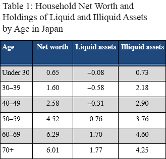
Note: The age of a household is indexed by the age of the household head. Liquid assets are net of all household borrowing, and net worth is the sum of liquid and illiquid assets. All numbers are divided by income of the 50–59 age group.
We expect that similar patterns also occur in other countries. However, the specific magnitudes of the age profiles of income, net worth, and their components will depend on institutions in a given country. For instance, households in countries that offer free tuition for higher education will have less student loan debt.
A tighter monetary policy (in other words, a higher policy nominal interest rate) is generally associated with higher real interest rates on deposits and loans (liquid assets), weaker performance of stock and real estate markets (illiquid assets), and slower growth in employment and wages. Given that the size and composition of income and net worth vary with age, one might surmise that a household's overall exposure to monetary policy also depends on its age. Retired households, for instance, may gain because they have no direct exposure to the labor market and hold large positive amounts of deposits whose return goes up. Young working-age households, in contrast, may lose because they have low net worth, loans, and low labor earnings.
Unfortunately, finding data that can be used to directly assess these hypotheses is challenging. In the United States, there is reasonably good survey data about how labor income and financial assets vary by age, but much less information about the size and value of household holdings of physical assets like homes, cars, and TV sets. Moreover, even in countries like Japan, where reasonably comprehensive survey data are available, a cross-sectional snapshot is produced only once every five years. Even if we can identify exogenous changes in monetary policy, we lack high-frequency data to measure how household exposures to monetary policy vary by age.
An alternative approach is to use an economic model. To see how this works, we define wealth as a household's net expected present value of future income from labor, assets, and the government. Wealth is an important economic concept because standard economic theory predicts that a household that sees its wealth increase from a tighter monetary policy will consume at least a fraction of its bonus. Conversely, a household whose wealth falls will consume less. Recent work by Auclert![]() builds on this insight. He uses a model to specify the dynamics of household income and decompose a household's consumption response to a change in monetary policy into four components:
builds on this insight. He uses a model to specify the dynamics of household income and decompose a household's consumption response to a change in monetary policy into four components:
- The income component captures the impact of changes in monetary policy on labor and government income.
- The unexpected inflation component captures net capital gains or losses associated with holdings of nominal assets. For instance, most government debt is nominally denominated, and a change in monetary policy affects the inflation rate and thus the real value of this nominal asset.
- The unhedged real interest rate component captures net real capital gains on household assets that are coming due at the time of the shock. For instance, a higher real return on deposits is good for a saver who has no loans, but a higher real interest rate can be bad for a borrower who enters the period with a maturing loan and faces a higher real cost of paying it off.
- Finally, the substitution component captures how a change in the interest rate affects a household's tradeoff between consuming today and saving today, which allows it to consume more tomorrow.
In our working paper, we propose a model designed to measure how household exposures to monetary policy vary over the life cycle. We specify the model to reproduce the main features about how household income, net worth, and portfolio allocations vary over the life cycle using data from Japan. Our model is rich in the sense that households are active for up to 100 years. They work and make asset-allocation decisions over time and interact in markets with households who have different ages and thus different asset-allocation priorities. Further, we model a government that taxes households, issues nominal debt, and runs a public pension program. Finally, the monetary authority sets the nominal interest rate on liquid assets using a simple rule. Fortunately, the model also has sensible implications for how nominal and real interest rates, wages, and government income respond to a tighter monetary policy.
Our model may sound rather sophisticated, but we make many simplifying assumptions. For instance, we are silent about what determines cross-sectional differences in income and wealth among households with the same age. In addition, households have only two assets that they can use to borrow or save. These simplifications make it easier to understand how age affects a household's exposure to monetary policy.
Figure 1 reports the age profile of household consumption responses to a surprise tightening in monetary policy in the year that monetary policy is tightened (left panel) and its decomposition into the four components we discussed above (right panel).
Note: The left panel is the sum of the four components, which is close to but not exactly the same as the age profile of consumption responses in the model.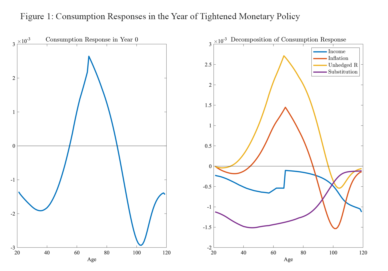
Source: Braun and Ikeda (2021)
The sign of the consumption response varies with age in figure 1. Households close to age 68 are increasing their consumption in response to higher wealth, while older retirees and younger working-age households are facing wealth losses. Another way to ascertain differences in exposure is to measure the magnitude of the consumption response. Households around age 30 reduce their consumption most, households close to the retirement age of 68 in the model increase their consumption most, and households that survive to about age 100 reduce their consumption. The magnitude of the consumption response is an imperfect measure of exposure because net worth also varies by age, as reported in table 1. In the model, the two groups who are reducing their consumption most have relatively low net worth. Younger workers are borrowers, and old retirees of age 100 have lived well beyond their expected life span and exhausted their savings. Thus, the biggest negative exposures to a tighter monetary policy in the model are among younger workers and oldest retirees.
The right panel of figure 1 reports the Auclert decomposition of consumption responses. For younger working-age households, the negative income component and the negative intertemporal substitution component are the two biggest factors. They have lower labor income and are at the age of their life cycle where they are accumulating assets, so movements in interest rates are particularly important for them. The other two factors are less important because their net worth is low. For households between 60 and 80, the income component is small, and the two asset-income components primarily drive their consumption responses. A lower inflation rate benefits this group because they are holding relatively large positive positions in nominally denominated liquid securities to provide for their retirement. The unhedged real interest rate component (unhedged R in the chart) is large because these households are savers and are at the stage of the life cycle where they draw down their assets to smooth their consumption during retirement.
In the model, life expectancy is 83 years, and households who survive beyond this age experience declines in all four components. They have been consuming their savings since age 68 and have low net worth. Also, some members of this group have debt. This age group also receives lower net income from the government. Government labor tax revenue is down and interest rate expenses on government debt are now higher so net government transfers to households fall, and this decline is significant for the oldest households in the model.
Taken together, these findings imply that inequality in net worth increases in the model in the year that monetary policymakers tighten policy. The highest net-worth age groups see their net worth increase, and the age groups with the lowest net worth see it fall. Consumption inequality also increases in the model because households with lower net worth tend to adjust their consumption by more than households with high net worth.
Hopefully, our findings have piqued your interest and left you with new questions. How large and persistent are the changes in inequality? What are the properties of an easier monetary policy? Does the amount of government debt in the economy matter? What about the effective lower bound on the nominal interest rate? I encourage you to read our working paper to find out.
I conclude with an old saying from economics: for each borrower, there is a lender. In our model, monetary policy alters interest rates, and a higher interest rate affects borrowers and lenders differently. It's a burden on younger working-age households and on the oldest retirees who are borrowers, but it's a boon for households close to age 68 who are the savers who provide the funding for the loans to the other two groups.
By  R. Anton Braun, a research economist and senior adviser in the Research Department at the Atlanta Fed